A Reformulation of Aumann-Shapley Random Order Values of Non-Atomic Games Using Invariant Measures

1 Introduction

A basic problem in cooperative game theory is to find rules for dividing the worth of the grand coalition among the players so that certain fairness is achieved. Mathematically, the problem is to find a mapping or an operator from the space of all set functions to the space of additive set functions satisfying certain desired properties. Using the linear vector space structure of the space of games, Shapley (1953) proved the existence and uniqueness of an operator satisfying certain axioms on fair division. The solution thus obtained is known as axiomatic value. Shapley also postulated an alternative set of fairness principles which come to be known as the random order value. In this approach, a player is given his expected marginal contribution in a random ordering of players, each ordering being equally likely among all possible orderings of the players. Shapley (1953) showed that the formulas for value from both approaches coincide.

The notion of Shapley value of non-atomic games has been used in designing fair cost allocations schemes and in studying the properties of market games. There have been several developments in the axiomatic value over the past several years, of which I point out briefly the ones relevant to our issues.¹ One most widely studied issue has been to find larger spaces of games on which an axiomatic value, possibly a unique one, exists. Robert J. Aumann and Shapley (1974) proved the existence of axiomatic value on pNA and bv$^{\prime }$NA (definitions of unknown terms in the introduction can be found in subsequent sections) and provided a ‘’diagonal formula’’ for games in pNA. The space pNA is economically the most important one which contains smooth market games and fair cost allocation schemes. The non-smooth games that arise from markets with strong complementarity, however, do not belong to the above spaces, nor even to the space ASYMP which is the largest space on which the value was shown to exist by Kannai (1966) (for more on this, see Robert J. Aumann and Shapley (1974)). Mertens (1988) extended the diagonal formula to a very large space, known as Mertens space, which includes these non-smooth games and the games from the above spaces. Using this formula Mertens proved the existence of the axiomatic value on the Mertens space.

Robert J. Aumann and Shapley (1974) proved that there does not exist an axiomatic value operator on all of BV. To have a value operator on all of BV, the symmetry axiom must be restricted to a proper subgroup. Ruckle (1982) has shown that when the symmetry is restricted to any “locally finite” group of automorphisms, there exists a value operator on all of BV. This result is further refined by Dov Monderer and Ruckle (1990). (D. Monderer 1989; Dov Monderer 1986) has shown that the non-atomic games that arise from smooth market economies have certain characteristics in which symmetry group could be restricted to appropriate subgroups of automorphisms.

The literature on extension of the random order value to the continuum case is very limited. Robert J. Aumann and Shapley (1974) initiated an extension by considering an set $\Omega$ of orderings of players that satisfy some measurability condition. They arrived at an Impossibility Principle: There does not exist a measure structure on $\Omega$ with respect to which a random order value could be assigned to games in pNA. In the light of this impossibility result, not much research has been directed along this line.

It is important to note that the main fairness property of the random order value arises from the fact that each player has an equal chance of forming a coalition with a set of players of any size and names, and random order value gives every player its unweighted average marginal contributions over all such coalitions. In the finite player case, the group of automorphisms of the players set and the set of orderings of players generated by the automorphisms are isomorphic, and thus the unweighted mean of the marginal contributions of a player over all orderings symmetrizes the mean with respect to the group of automorphisms. That is, the expected value of random marginal contribution set function becomes invariant with respect to the group of automorphisms. Raut (2003) has shown that on the space of games with a finite set of players, the expected value (i.e., the mean) of the marginal contributions of a player is symmetric with respect to a group of automorphisms if and only if the randomness of the orders is induced by the automorphism group assigning equal likelihood to each order (i.e., if and only if the mean is unweighted). I use these insights from finite games to reformulate the random order approach to values of games with a continuum of players. Raut (1997) was the first attempt in extending the random order approach to values of non-atomic games along this line. Furthermore, Raut (1997) has constructed an invariant measure structure on an uncountably large group of Lebesgue measure preserving automorphisms. The random order value with respect to this invariant automorphism group coincides with the fully symmetric Aumann-Shapley axiomatic value for a large class of games. In this paper, I provide a general formulation of this approach and prove further results.

In Section 2, I lay out the basic framework for the reformulation and point out the differences between the present approach with the Aumann-Shapley approach. In Section 3, I show that the reformulated approach is valid. In Section 4, I discuss issues concerning the choice of a symmetry group, and sketch the construction of the invariant probability measurable group $\breve{\Theta}$ as projective limit group that was studied in more details in Raut (1997). In this section I also provide further results on the projective limit group $\breve{\Theta}$ and the random order value operator with respect to $\breve{\Theta}$. I relegate most of the remarks to Section 5.

2 The Basic Framework

I adopt the convention of using a subscripted notation $\mathcal{B}_{X}$ to denote a Borel $\sigma$-algebra of a topological space X (i.e., the $\sigma$-algebra generated by the class of open sets of X) and to denote any general $\sigma$-algebra, I do not use a subscript. Let $I=[0,1]\subset \Re$ be the set of players. Let $\mathcal{B}_{I}$ be the Borel $\sigma$-algebra of $I$. The elements of $\mathcal{B}_{I}$ are the set of admissible coalitions. A game is a set function $V:\mathcal{B}_{I}\to \Re$ such that $V(\emptyset )=0$. Let $G_{I}$ be the set of all games. Let FA be the set of finitely additive set functions on $(I,\mathcal{B}_{I})$. A measure is a countably additive set function. One can check easily that $G_{I}$ and FA are linear vector spaces. A game V is monotonic if $V(S)<V(T)$ for any $S,T\in \mathcal{B}_{I}$, $S\subset T$. A Borel automorphism is a measurable map $\theta :(I,\mathcal{B}_{I})\to (I,\mathcal{B}_{I})$ such that it is one-one, onto and $\theta ^{-1}$ is also measurable. Let $\mathcal{G}$ be the set of all Borel automorphisms on $(I,\mathcal{B}_{I})$. One can check that $\mathcal{G}$ is a non-commutative (also known as non-abelian) group with the composition of functions as the group multiplication operation and the identity function as the group identity.

For each $\theta \in \Theta$, define the linear operator $\ddot{\theta}:G_{I}\to G_{I}$ by

$$(\ddot{\theta}V)(S)=V(\theta ^{-1}(S)), \forall S\in \mathcal{B}_{I}.$$

Given a subgroup of automorphisms, $\Theta \subset \mathcal{G}$, a linear subspace $Q\subset G_{I}$ is said to be $\Theta$-symmetric if $\ddot{ \theta}Q\subset Q$ for all $\theta \in \Theta$. Let Q be a linear subspace of $G_{I}$. An operator $\Phi :Q\to FA$ is said to be linear if $\Phi (\alpha V_{1}+V_{2}) = \alpha \Phi (V_{1})+\Phi (V_{2}) \forall V_{1},V_{2}\in Q,\alpha \in \Re$. $\Phi$ is said to be positive if the set function $(\Phi V)$ is monotonic for any monotonic $V$ in the domain of $\Phi .$ The operator $\Phi$ is said to be efficient if $\Phi V(I)=V(I) \forall V\in Q$. For a $\Theta$-symmetric space $Q$, the operator $\Phi :Q\to FA$ is said to be a $\Theta$-symmetric operator if $\Phi \ddot{\theta}V=\ddot{\theta}\Phi V, \forall \theta \in \Theta ,V\in Q$.

I introduce a more general notion of value operator: A $\Theta$-symmetric axiomatic value operator on a $\Theta$-symmetric linear space of games $Q$ is a positive, linear, efficient, and $\Theta$-symmetric operator $\Phi :Q\to FA$. Note that a $\mathcal{G}$-symmetric axiomatic value operator is the same as the original Aumann-Shapley axiomatic value operator.

Although for the random order approach of this paper, I do not need to impose any topological structure on the space of games, to relate my results to the literature, I restate the following topological concepts from Robert J. Aumann and Shapley (1974). A game $V$ is of bounded variation if there exist monotonic games $U$ and $W$ such that $V=U-W$. Denote by BV the set of all games of bounded variation. It is known that BV is a linear vector space over $\Re$. Define a map $\parallel . \parallel _{BV}: BV \to \Re$ by

$$\parallel V\parallel _{BV}=inf\left\{ U(I)+W(I) V=U-W, U\text{ and }W\text{ are monotonic games}\right\}$$

for each $V\in$ BV. It can be shown that $\parallel .\parallel _{BV}$ is a well defined norm on BV and with this norm BV is a Banach space, see Robert J. Aumann and Shapley (1974), Corollary 4.2, and Proposition 4.3. The following notation is standard in the literature:

$$\begin{aligned} NA &=\text{ the set of non-atomic measures on }\left( I,\mathcal{B}_{I}\right) \\ NA^{1} &=\text{ the set of non-atomic probability measures on }\left( I,\mathcal{B}_{I}\right) \\ pNA &=\Vert .\Vert _{BV}-\text{closure of the linear space spanned by the powers of }\mu \in NA^{1} \\ bv^{\prime }NA &=\Vert .\Vert _{BV}-\text{closure of the linear space spanned by }f\circ \mu \in NA^{1}\text{, where }f:I\rightarrow \Re \\ &\text{is of bounded variation, continuous at 0 and 1, and }f(0)=0. \end{aligned}$$ It is known that FA, NA and pNA are all closed subspaces of BV.

2.1 Generation of Random orders

Two features of the random order approach to values of games with finite set of players that I adopt to the present context are: First, each automorphism ² generates a distinct ordering of players, i.e., the set of orders is the same as the group of automorphisms. Second, for all games, the mathematical expectation of the random marginal contribution set function is symmetric with respect to the group of automorphisms if and only if each random ordering of players is equally likely (see Raut (2003)). In the finite players case, the main reason why the expected marginal contribution set function becomes symmetric for any game and with respect to the full group of permutations is that every player is equally likely to form a coalition with a set of players of any size and names in a random order. I adopt these two features to the continuum case.

Note that each $\theta \in \Theta$ generates a binary relation, $\succ _{\theta }\subset I\times I$ defined by

$$\text{ for any }s,t\in I, s\succ _{\theta }t \Leftrightarrow \theta (s)>\theta (t).$$

Recall that an order $\succ$ on a set $X$ is a linear order, which is also known as total order, if for any $x,y\in X$, $x\ne y$, either $x\succ y$ or $y\succ x$, for no $x\in I$, $x\succ x$, and for any $x,y,z \in I$, $x\succ y$, $y\succ z$ $\Rightarrow$ $x\succ z$. A total order in this paper is referred to as an order. It is easy to verify that the binary relation $\succ _{\theta }$ generated by an automorphism $\theta$ is an order on $I.$ Let $\bar{I}=I\cup \{\infty \}.$ Extend the domain of each $\theta \in \mathcal{G}$ from $I$ to $\bar{I}$ by assigning $\theta (\infty )=\infty .$ For an order $\succ _{\theta }$, $\theta \in \mathcal{G}$, and a $s\in \bar{I}$, define an initial segment $I(s,\theta )$ by $I(s,\theta) = {t\in I| \theta (s)>\theta (t)}$. The set $I(s,\theta)$ is viewed as the set of players who are before player $s$ in the order $\succ _{\theta }$.

Unlike the finite player case, two Borel automorphisms in the continuum case, however, may generate the same ordering of $I$. For instance, take two automorphisms $\theta$ and $e\in \mathcal{G},$ defined by $\theta (x)=x^{2}$ , $x\in I$ and $e(x)=x,x\in I$. Both generate the order $\succ _{e}$. Thus the set of orderings of players and the group of Borel automorphisms of players are not isomorphic. I derive the set of orders $\Omega$ generated by a group of automorphisms $\Theta$ as follows:

Define an equivalence relation $\sim$ on $\Theta \times \Theta$ by,

$$\theta _{1}\sim \theta _{2},\text{ for }\theta _{1},\theta _{2}\in \Theta \Leftrightarrow \theta _{1},\theta _{2}\text{ generate the same order on }I.$$

Let $\Theta _{e}=\left\{ \theta \in \Theta |\theta \sim e\right\}$. It can be easily shown that $\Theta _{e}$ is a subgroup of $\Theta$ and the set of distinct orders, $\Omega$, generated by the automorphisms in $\Theta$ is the set of right cosets given by

$$\Omega \equiv \Theta /\Theta _{e}\equiv \left\{ \Theta _{e}\theta \theta \in \Theta \right\}$$

In the finite player case, the set of automorphisms of players is finite and for finite sets the concept of equal likelihood is obvious. In the continuum case, however, the set of automorphisms of the players is uncountable. The analogue of the equal likelihood in the continuum case is the following concept of an invariant measure, which requires the underlying space to have a group structure:

Definition 1 A measure space $\left( \Theta ,\mathcal{A},\Gamma \right)$ is said to be an invariant measurable group if $\Theta$ is a group, the map $(\theta _{1},\theta _{2})\rightarrow \theta _{1}\theta _{2}^{-1}$ from $\left( \Theta \times \Theta ,\mathcal{A}\times \mathcal{A}\right)$ onto $\left( \Theta ,\mathcal{A}\right)$ is measurable, and $\Gamma$ is $\sigma$-finite, not identically zero, and right invariant, i.e., $\Gamma (E\theta )=\Gamma (E)$, for all $E\in A$, and $\theta \in \Theta$, where $E\theta \equiv \left\{ \sigma \theta |\sigma \in E\right\}$. $\Gamma$ is known as a right invariant measure.³ When $\Gamma$ is furthermore a probability measure, a measurable group $\left(\Theta ,\mathcal{A},\Gamma \right)$ is said to be a right invariant probability measurable group.

In general $\Theta _{e}$ is not a normal subgroup⁴ of $\Theta$ and hence $\Omega$ is not necessarily a group. To see this, consider two automorphisms $\theta \in \mathcal{G}$ and $\theta _{e}\in \Theta _{e}$ defined by

$$\begin{aligned} \theta (x) &=\left\{ \begin{array}{ll} 1-x & if 0\le x<1/2 \\ x-1/2 & if 1/2\le x\le 1 \end{array} \right. \\ \theta _{e}(x) &=\left\{ \begin{array}{ll} 0.01x & if 0\le x<0.8 \\ 0.008+4.96(x-0.8) & if .8\le x\le 1. \end{array} \right. \end{aligned}$$

Let $t=0.4$ and $s=0.3$. Thus $\theta _{e}(s)<\theta _{e}(t)$, but $(\theta ^{-1}\theta _{e}\theta )(s)=0.507>0.506=(\theta ^{-1}\theta _{e}\theta )(t)$, thus $\theta ^{-1}\theta _{e}\theta \notin \Theta _{e}$.

Thus, the set of orders $\Omega$ does not inherit a group structure that can be used to extend the concept of equal likelihood of orderings in $\Omega$. But $\Omega$ is a homogeneous space acted on by the group $\Theta$, and for homogeneous spaces there is a natural concept of invariant measure (see Section 55 in Parthasarathy (1977), or Section 7.4 in Segal and Kunze (1968)). In the present set-up, however, I can use the natural map $\Pi :\Theta \to \Omega$ defined by $\Pi (\theta )=\Theta _{e}\theta$ to induce an invariant probability measure structure $\left( \Omega ,\mathcal{B},\mu \right)$ on the homogeneous space $\Omega$ of induced orders. The measure space of orders $\left( \Omega ,\mathcal{B},\mu \right)$ will be referred to as a set of random orders.

2.2 Connection with Aumann-Shapley measurable orders

In this section I study the relationship between the notion of orders used in this paper and the notion used in Robert J. Aumann and Shapley (1974), pp.94-95. Aumann and Shapley defined an order $\mathcal{R}$ on $I$ to be $measurable$ if the $\sigma$-algebra generated by the set of initial segments $\{I(s, \mathcal{R})|s\in \bar{I}\}$ coincides with $\mathcal{B}_{I}$. An order $\succ _{\theta}$ generated by a Borel automorphism $\theta \in \mathcal{G}$ is measurable in the Aumann-Shapley sense, but not every order measurable in the Aumann and Shapley sense can be represented by a Borel automorphism. To see this, let $u:I\to I\cup \{2\}$ be a Borel isomorphism⁵ and define an order $\succ _{u}$ on $I$ by $x,y\in I$, $x\succ _{u}y$ $\Leftrightarrow$ $u(x)>u(y)$. It is easy to see that $\succ _{u}$ is an Aumann-Shapley measurable order but it cannot be induced by an automorphism. The difference between an Aumann-Shapley measurable order and an order generated by an automorphism can be seen from the complete characterization of both types of orders in Proposition 1 below.

An order $\succ$ is said to be strongly separable if there is a countable set $Z\subset I$ so that for any $x,y\in I$, $x\succ y$, implies that there is a $z\in Z$ and $x\succ z\succ y$. An order $\succ$ is said to be a complete order⁶ if any non-empty subset of $E\subset I$, which is bounded above, has a least upper bound ($l.u.b.$) in $I$. An order $\succ$ is said to be weakly separable if there is a countable set $Z\subset I$ so that for any $x,y\in I$, $x\succ y$, implies that there is a $z\in Z$ and $x\succeq z\succeq y$.

Proposition 1

• 1. An order $\succ$ on $I$ arises from a Borel automorphism if and only if $\succ$ is strongly separable and complete.
• 2. An order $\succ$ on I is Aumann-Shapley measurable if and only if $\succ$ is weakly separable and all initial segments are measurable.

Proof. [Proof of Proposition 1:] Part (i): Let $\succ$ on $I=[0,1]$ be a strongly separable complete order. Let $Z\subset I$ be the countable set in the definition of strong separability of $\succ .$ Let $\succ _{e}$ denote the standard order on $I$. Let $Q_{I}$ be the set of rational numbers that lie in $(0,1)$. It is well known that $\succ _{e}$ is strongly separable on $(0,1)$ with respect to $Q_{I}$, and that $(0,1)$ is complete. For ease of exposition, let $(X,\succ )$ denote the set $X$ ordered by $\succ .$ Let $\dot{I}$ denote the ordered set $(I,\succ )$ after its first and last ordered elements being removed. Without loss of generality, I assume that $Z\subset \dot{I}$. An order isomorphism between two ordered sets is a one-one and onto map between the sets which preserves the orders of the sets. By Cantor’s theorem it is known that there exists an order isomorphism $h:\left( Z,\succ \right) \to \left( Q_{I},\succ _{e}\right)$. For each $x\in \left( \dot{I},\succ \right)$, let $R(x)=\left\{ h(z)|z\in Z\text{ and }x\succ z\right\}$ which is a subset of $Q_{I}$. It is easy to note that $R(x)$ is non-empty and bounded above, and hence has a $l.u.b.$ Define the map $f:\dot{I}\to (0,1)$ by $f(x)\equiv l.u.b.R(x)$. Strong separability of $\succ$ implies that $f$ is order preserving and hence one-one. Completeness of $\succ$ implies that $f$ is a onto map. Now I extend the map $f$ to $\left( I,\succ \right)$ by letting it map the first and last elements of $\left( I,\succ \right)$ respectively to 0 and 1. Notice that the initial segments $I(s,\succ )$, $s\in \bar{I}$ under the order $\succ$ are all of the form $I(s,\succ )=f^{-1}[0,x)$, where $x=f(s)$. Hence, these initial segments generate $\mathcal{B}_{I}$ and $f^{-1}$ is measurable. Since $f$ is one-one, the Borel isomorphism theorem assures that $f$ is measurable, and hence $f$ is a Borel automorphism.

Conversely, an order generated by a Borel automorphism is clearly strongly separable and complete. To see this, let $\theta$ be an automorphism. Taking $Z=\theta ^{-1}\left( Q_{I}\right)$ in the definition of strong separability, it is easy to note that $\succ _{\theta }$ is strongly separable. For any non-empty $E\subset \left( I,\succ _{\theta }\right)$ one can show that $\theta ^{-1}\left( \sup_{t\in E}\theta (t)\right)$ is the $l.u.b$ of $E$.

Proof of part (ii) follows from Robert J. Aumann and Shapley (1974), p.107. %

$\blacksquare$

2.3 $\Theta$-symmetric random order value operator

I now introduce the notion of $\Theta$-symmetric random order value operator. Given a game $V$, and an order $\succ _{\theta }$, $\theta \in \mathcal{G}$, define a marginal contribution set function, $\phi ^{\theta }V$ on $(I,\mathcal{B}_{I})$ as a measure on $(I,\mathcal{B}_{I})$ such that $$\left( \phi ^{\theta }V\right) (I(s,\theta ))=V(I(s,\theta )), \forall s\in \bar{I}. \tag{1}$$

Notice that for any $\theta ,\theta ^{\prime }\in \Theta$ such that $\theta \sim \theta ^{\prime }$, we have $I(s,\theta )=I(s,\theta ^{\prime })$. Hence it follows from Equation 1 that $\phi ^{\theta }V(S)=\phi ^{\theta ^{\prime }}V(S)$ for all $S\in \mathcal{B}_{I}$. This allows us to unambiguously define $(\phi ^{\omega }V)(S)=(\phi ^{\theta }V)(S)$ where $\theta$ is such that $\omega =\Theta _{e}\theta$.

Let $\Phi _{\Gamma }$ be an operator that associates to each game $V$ its expected marginal contribution set function defined by

$$\begin{aligned} (\Phi _{\Gamma }V)(S) &\equiv \int_{\Omega }(\phi ^{\omega }V)(S)d\mu (\omega ) \nonumber \\ &=\int_{\Theta }(\phi ^{\theta }V)(S)d\Gamma (\theta ), S\in \mathcal{B}_{I}. \end{aligned} \tag{2}$$

The second equality follows from the change of variable formula for Lebesgue integrals and the facts in the previous paragraph. Define the space of games:

$$L1(\Theta ,\Gamma )=\left\{ V\in G_{I} \phi ^{\theta }V(S) \text{ is integrable for all }S\in \mathcal{B}_{I}\right\} . \tag{3}$$

Definition 2 Let $\Theta \subset G$ be a given subgroup of automorphisms and $Q\subset G_{I}$ be a linear space of games. The operator $\Phi _{\Gamma }:Q\rightarrow FA$ defined in Equation 2 with respect to an invariant probability measurable group structure $\left( \Theta ,\mathcal{A},\Gamma \right)$ on $\Theta$ such that $Q\subset L1(\Theta ,\Gamma )$ is said to be a $\Theta$-symmetric random order value operator on $Q$.

In the next section, I will first prove a few basic properties of $\Phi _{\Gamma }$ and $L1(\Theta ,\Gamma )$ to establish that these two objects render a valid approach to random order value.

3 The operator $\Phi_\Gamma$ is a valid random order value operator

For the operator $\Phi_\Gamma$ defined in Equation 2 to yield a random order value operator, three basic facts must be established. First, for any game $V$ and any order $\succ _{\theta }$, $\theta \in \Theta$, if there exists a measure $\phi ^{\theta }V$ satisfying Equation 1, it should be unique so that for each $S\in \mathcal{B}_{I}$, $\phi ^{\theta }V(S)$ is a function of $\theta$. Proposition 2 ensures this. Second, in order for the operator $\Phi _{\Gamma }$ to be $\Theta$-symmetric with respect to a given subgroup of automorphisms $\Theta$, the linear space $L1(\Theta ,\Gamma )$ defined in Equation 3 must be a $\Theta$-symmetric linear subspace of $G_{I}$. This is shown to be true in Proposition 4. Third, the approach is of little use if for a given symmetry group of automorphisms $\Theta$, two different invariant probability measure structures on it assign two different finitely additive set functions as mathematical expectations of the random marginal contribution set function of a game. The second part of Theorem 1 ensures that the mathematical expectation in Equation 2 depends only on the group of automorphisms $\Theta$ but not on a specific invariant probability measurable group structure on $\Theta$. I introduce the following concept to be used through out the paper.

Definition 3 A set function $V\in G_{I}$ is said to be normalized set function if (i) $V(A_{n})\rightarrow 0$ as $n\rightarrow \infty$ for any sequence of sets, $A_{n}\in B_{I}$, $A_{n}\downarrow \emptyset$ as $n\rightarrow \infty$, and (ii) $V(A_{n})\rightarrow V(A)$ as $n\rightarrow \infty$ for any sequence of sets, $A_{n} \in B_{I}$, $A_{n}\uparrow A$ as $n\rightarrow \infty$, where $A\in B_{I}$.

Denote by $NBV$ the set of normalized set functions from BV. It is easily seen that $NBV$ is a linear space.

For Equation 2 to be meaningful, the following proposition proves that the marginal contribution set function $\phi ^{\theta }V$ is unique so that it is a function of $\theta$ not a correspondence, and provides conditions under which $\phi ^{\theta }V$ exists for all $\theta \in \mathcal{G}$ for a large class of games in BV. The second part of Proposition 2 is used to prove Theorem 4 later.

Proposition 2

• 1. For a game $V$ in $G_{I}$ and an order $\succ_{\theta }$, $\theta \in G$, if a marginal contribution set function $\phi ^{\theta }V(S),S\in B_{I}$ exists, it is unique.
• 2. For any $V\in$ NBV, and for any $\theta \in G$, the marginal contribution set function, $\phi ^{\theta }V$ exists and it is countably additive; furthermore, for each $\theta \in G$, $\phi ^{\theta }:$ NBV $\rightarrow$ NBV is a bounded linear operator in the $\Vert .\Vert _{BV}$ norm on NBV and for $V\in$ NBV, $\Vert \phi ^{\theta }V\Vert _{BV}\leq \Vert V\Vert _{BV}$ uniformly for all $\theta \in G$.

Proof. Let us denote by $[s,t)_{\theta }=\{j\in I | \theta (s)\le \theta (j)<\theta (t)\}$. Denote by $\mathcal{D}_{\theta }=\left\{[s,t)_{\theta } | s\in I,t\in \bar{I}\right\}$. One can easily verify that $\mathcal{D}_{\theta }$ is the smallest Boolean semi algebra containing all initial segments $\mathcal{I}_{\theta }=\left\{ I(s,\theta ) | s\in \bar{I}\right\}$. Without loss of generality, assume that V is monotonic. There is a unique extension of $\phi ^{\theta }V$ from $\mathcal{I}_{\theta }$ to $\mathcal{D}$$_{\theta }$ such that $\phi ^{\theta }V$ is finitely additive on $\mathcal{D}_{\theta }$ and Equation 1 is satisfied. More precisely, note that for the initial segments in $\mathcal{D}_\theta$, Equation 1 defines $\phi ^{\theta }V$, and for all other sets in $\mathcal{D}_{\theta },$ there is only one way $\phi ^{\theta }V$ can be defined as follows: $$(\phi ^{\theta }V)\left( [s,t)_{\theta }\right) =V\left( I(t,\theta )\right) -V\left( I(s,\theta )\right) \text{ for }s\in I\text{ and }t\in \bar{I}.$$ It is known that such a $\phi ^{\theta }V$ can be uniquely extended to a measure on $\mathcal{B}_{I}$ (see, for instance, Parthasarathy (1977), Corollary 16.9).

I now prove part (ii) of the proposition. For any $\theta \in \mathcal{G}$, define the real valued function $F_{\theta }:\bar{I}\to \mathcal{R}$ by $F_{\theta }(x)=V\left( \theta ^{-1}\left( [0,x)\right) \right)$. Note that for any sequence of real numbers $x_{n},$ $n\ge 0$ from $\bar{I}$ such that $x_{n}\downarrow 0$, we have $\theta ^{-1}[0,x_{n})\downarrow \emptyset$ as $n\to \infty$, and since $V\in$ $NBV$, it follows that $F_{\theta }(x_{n})=V\left( \theta ^{-1}\left( [0,x_{n})\right) \right) \to 0$ as $n\to \infty$. Similarly, for any sequence of real numbers $x_{n}\uparrow x$ in $\bar{I}$, we have $F_{\theta }(x_{n})\to F_{\theta }(x)$. Hence by Theorem 8.14 in Rudin (1987), there exists a unique signed measure $\lambda _{\theta}$ on $\mathcal{B}_{I}$ such that

$$\lambda _{\theta }\left( [0,t)\right) =F_{\theta }(t) \forall t\in \bar{I}.$$ Taking $t=\theta (s)$, $s\in \bar{I}$, noting that $I(s,\theta )=\theta ^{-1}[0,\theta (s))$, and defining the measure $\phi ^{\theta }V$ on $\mathcal{B}_{I}$ by $\left( \phi ^{\theta }V\right) \equiv \lambda _{\theta }\theta ^{-1}$, we get $$\left( \phi ^{\theta }V\right) \left( I(s,\theta )\right) =V\left( I(s,\theta )\right) \forall s\in \bar{I}.$$ Hence, there exists a unique (uniqueness follows from part (i) of the proposition) marginal contribution measure for $\theta \in \mathcal{G}$. It is easy to check that $\phi ^{\theta }:$ $NBV\to NBV$ is linear. Since orders generated by automorphisms are also Aumann-Shapley measurable orders, the rest of the proposition follows from their Proposition 12.8.

$\blacksquare$

The second part of Proposition 2 establishes that the marginal contribution set function is a measure. The following proposition shows the algebraic interplay of a game $V$ and the actions of any subgroup of automorphisms $\Theta$ in the arguments, $\theta ,V,S$, of the marginal contribution measure $(\phi ^{\theta }V)(S)$. The second part of the proposition provides a computational formula for the marginal contribution measure for a large class of scalar measure valued games. First part of Proposition Proposition 3 is used to prove the $\Theta$-symmetry of the linear space of games $L1(\Theta ,\Gamma )$ in Proposition Proposition 4, and the $\Theta$-symmetry of the operator $\Phi _{\Gamma }$ in Theorem 1; the second part of Proposition 3 is used to establish the diagonal formula Equation 9 in Theorem 5.

Proposition 3

• 1. Let $\Theta$ be any fixed subgroup of automorphisms in $G$. Suppose for a game $V\in G_{I},$ the marginal contribution measure $\phi ^{\theta }V$ exists for all $\theta \in \Theta$. Then for any $\pi \in \Theta$, the marginal contribution measure $\phi ^{\theta }(\ddot{\pi}V)$ for the game $\ddot{\pi}V$ also exists for all $\theta \in \Theta$, and it is related to the marginal contribution measure of $V$ by,
     $$\phi ^{\theta }(\ddot{\pi}V)(S)=(\phi ^{\theta \pi }V)\left( \pi ^{-1}(S)\right) ,\forall S\in \mathcal{B}_{I}. \tag{4}$$
• 2. Let $f:I\rightarrow \Re$ be an absolutely continuous function, and $\theta$ be any Lebesgue measure preserving automorphism on $I$, then the marginal contribution measure of the scalar measure valued game $f\circ \lambda$ is given by:
     $$\phi ^{\theta }(f\circ \lambda )\left( S\right) =\int_{S}f^{\prime }\left( \theta (t)\right) d\lambda (t). \tag{5}$$

The following lemma will be used to prove Proposition 3 and other results:

Lemma 1 Let $S\subset \Re$. Suppose $\theta: S \rightarrow S$, and $\pi :S \rightarrow S$ be two automorphisms of $S$. Denote by $I(s,\theta )=\{t\in S | \theta (t)<\theta (s)\}$ for any automorphism $\theta$. Then, $\pi ^{-1}\left( I(s,\theta )\right) =I\left( \pi ^{-1}(s),\theta \pi \right)$.

Proof. The result follows from the following equivalent statements:

$$\begin{aligned} x\in \pi ^{-1}\left( I(s,\theta )\right) &\Leftrightarrow \pi (x)\in I\left( s,\theta \right) \\ &\Leftrightarrow \theta (\pi (x))<\theta (s) \\ &\Leftrightarrow (\theta \pi )(x)<(\theta \pi )\pi ^{-1}(s) \\ &\Leftrightarrow x\in I\left( \pi ^{-1}(s),\theta \pi \right) . \end{aligned}$$

$\blacksquare$

Proof. [Proof of Proposition 3:] To prove part (i) note that for any $s\in I,$ $$\begin{aligned} (\phi ^{\theta }(\ddot{\pi}V))(I(s,\theta )) &=(\ddot{\pi}V)(I(s,\theta ))\text{ by definition of }\phi ^{\theta } \\ &=V\left( \pi ^{-1}I(s,\theta ) \right) \text{ by definition of }\ddot{\pi} \\ &=V\left( I\left( \pi ^{-1}(s),\theta \pi \right) \right) \text{ ... (1) } \\ &=(\phi ^{\theta \pi }V)\left( I(\pi ^{-1}(s),\theta \pi )\right) \text{ by definition of }\phi ^{\theta \pi } \\ &=((\phi ^{\theta \pi }V)\pi ^{-1})\left( I(s,\theta )\right) \text{ ...(2) } \end{aligned}$$ Steps (1) and (2) follow from Lemma 1. Since the equality holds for all the initial segments in $\mathcal{I}_{\theta }$, they agree on $\mathcal{B}_{I}$. Thus the measure $(\phi ^{\theta }\ddot{\pi}V)$ exists whenever the measure $(\phi ^{\theta \pi }V\pi ^{-1})$ exists. Since $\theta \pi \in \Theta$, by the hypothesis of the Proposition, $(\phi ^{\theta \pi }V)$ exists. But $(\phi ^{\theta \pi }V)\pi ^{-1}$ is a measure whenever $(\phi ^{\theta \pi }V)$ is a measure. Hence I conclude that $\phi ^{\theta }(\ddot{\pi}V)$ exists for all $\theta \in \Theta$ and is given by the right hand side of Equation 4.

Part (ii) of the Proposition follows from Proposition 5 in Raut (1997).

$\blacksquare$

Proposition 4 The space of games $L1(\Theta ,\Gamma )$ is a $\Theta$-symmetric linear subspace of $G_{I}$.

Proof. [Proof of Proposition 4:] It is easy to check that $L1(\Theta ,\Gamma )$ is a linear space. I shall show that it is $\Theta$-symmetric. Let $\pi \in \Theta$, and $V\in L1(\Theta ,\Gamma )$. I want to show that $\ddot{\pi}V\in L1(\Theta ,\Gamma )$. From Proposition 3(i), it is clear that $\phi ^{\theta }(\ddot{\pi}V)(S)$ exists for all $\theta \in \Theta$ and $S\in \mathcal{B}_{I}$ and is given by ($\phi ^{\theta \pi }V)\left( \pi ^{-1}(S)\right)$. But since $\left( \Theta ,\mathcal{A},\Gamma \right)$ is an invariant probability measurable group, it has the property that for any fixed $\pi \in \Theta$ if $h(\theta )$ is integrable, then the right translation of the function $h(\theta \pi )$ is also integrable and both have the same integral. Since $(\phi ^{\theta }V)\left( \pi ^{-1}(S)\right)$ is integrable by assumption, it follows therefore that $\ddot{\pi}V\in L1(\Theta ,\Gamma)$.

$\blacksquare$

Theorem 1 below assures that the operator $\Phi_\Gamma$ defined in Equation 2 is independent of a specific invariant probability measurable group structure on $\Theta$ and it coincides with the $\Theta$-symmetric axiomatic value operator on $a$ space of games. In fact, a $\Theta$-symmetric random order value operator is a particular characterization of the $\Theta$-symmetric axiomatic value operator.

Theorem 1 Let $\left( \Theta ,\mathcal{A},\Gamma \right)$ be an invariant probability measurable group structure on a fixed subgroup of automorphisms $\Theta \subset G$. Then the operator $\Phi _{\Gamma }$ defined in Equation 2 is positive, linear, efficient and $\Theta$ -symmetric on $L1(\Theta ,\Gamma )$ or any $\Theta$-symmetric linear subspace of $L1(\Theta ,\Gamma )$. Furthermore, suppose $\left( \Theta , \mathcal{A}^{\prime },\Gamma ^{\prime }\right)$ is another invariant probability measurable group structure on $\Theta$, then $\Phi _{\Gamma }=\Phi _{\Gamma ^{\prime }}$ on the linear space of games $L1(\Theta ,\Gamma )\cap L1(\Theta ,\Gamma ^{\prime })$.

Proof. It is easy to see that $\Phi _{\Gamma }$ is linear, positive and efficient. I want to show that the right invariance of $\Gamma$ implies $\Theta$-symmetry of $\Phi _{\Gamma }.$ To that end, note that $$\begin{aligned} \Phi _{\Gamma }(\ddot{\pi}V)(S) &=\int_{\Theta }\phi ^{\theta }(\ddot{\pi}V)(S)d\Gamma (\theta ) \\ &=\int_{\Theta }(\phi ^{\theta \pi }V)\left( \pi ^{-1}(S)\right) d\Gamma (\theta ), \text{...(1) } \\ &=\int_{\Theta }(\phi ^{\theta \pi }V)\left( \pi ^{-1}(S)\right) d\Gamma (\theta \pi )\text{ since }\Gamma \text{ is right invariant} \\ &=(\Phi _{\Gamma }V)(\pi ^{-1}(S)) \\ &=\ddot{\pi}(\Phi _{\Gamma }V)(S), S\in \mathcal{B}_{I}\text{ and }V\in L1(\Theta ,\Gamma ). \end{aligned}$$ Step (1) follows from Proposition 3(i). Hence, $\Phi _{\Gamma }\ddot{\pi}=\ddot{\pi}\Phi _{\Gamma }$.

To prove the second part of the theorem, suppose $V\in L1(\Theta ,\Gamma )\cap L1(\Theta ,\Gamma ^{\prime })$. Then $\phi ^{\theta }V$ is measurable with respect to the invariant $\sigma$-algebra $\mathcal{A}_{0}=\mathcal{A} \cap \mathcal{A}^{\prime }$, and furthermore, the expected value of the marginal contribution set function $(\phi ^{\theta }V)(S)$ will be the same with respect to $\left( \Theta ,\mathcal{A},\Gamma \right)$ and $\left( \Theta ,\mathcal{A}_{0},\Gamma _{0}\right)$ where $\Gamma _{0}$ is the restriction of $\Gamma$ on $\mathcal{A}_{0}$. Note that $\mathcal{A}_{0}$ is an invariant $\sigma$-algebra on $\Theta$ and we have two probability measures $\Gamma _{0}$ and $\Gamma _{0}^{\prime }$ which are respectively the restrictions of $\Gamma$ and $\Gamma ^{\prime }$ to $\mathcal{A}_{0}$. Hence, an application of Theorem B, Section 60 in Halmos (1950), taking his E to be the whole set $\Theta$ yields $\Gamma _{0}(F)=\Gamma _{0}^{\prime }(F)$ for all $F\in \mathcal{A}_{0}$. Thus, the expected values of $\left( \phi ^{\theta }V\right) (S)$ with respect to both invariant probability measurable group structures, $\left( \Theta ,\mathcal{A},\Gamma \right)$ and $\left( \Theta ,\mathcal{A}^{\prime },\Gamma ^{\prime }\right)$ are the same.

$\blacksquare$

4 On the choice of a symmetry group

In the previous section I have established that given any set of automorphisms with an invariant probability measurable group structure on it, there exists a random order value operator on the space consisting of games for which the mathematical expectations of the random marginal contribution measure are finite. (D. Monderer 1989; Dov Monderer 1986) has provided economic situations that lead to restricting the symmetry group. I provide some technical grounds for restricting the symmetry group. Three aspects of the invariant automorphism group that matter for our approach are (1) the characteristics of the automorphisms that are members of the group, (ii) the size of the automorphism group, and (iii) the fineness of the $\sigma$-algebra on it.

The type of automorphisms that are members of the group matters because these member automorphisms determine what kind of players are equally likely to be placed before a given player. This beckons us to consider the strongly mixing automorphisms. To fix ideas, consider mixing with respect to the Lebesgue measure $\lambda$. A Lebesgue measure preserving automorphism $\theta \in \mathcal{G}$ is said to be strongly mixing if $\lim_{n\to \infty }\lambda \left( \theta ^{-n}E\cap F\right) =\lambda \left( E\cap F\right)$ for all $E,F\in \mathcal{B}_{I}$. In essence, a strongly mixing automorphism $\theta$ allows thorough mixing of any set of players $t\in E$ with any other player in the unit interval $I$ by producing an orbit $\mathcal{Q}(E)=\left\{ \theta ^{n}t|t\in {E},n=0,1,..\right\}$ which is dense and uniformly spread allover $I$. A Lebesgue measure preserving automorphism is weakly mixing if $\lim_{n\to \infty }\frac{1}{n}\sum_{j=1}^{n}\lambda \left( \theta ^{-j}E\cap F\right)$ $=$ $\lambda \left( E\cap F\right)$. It is known that with respect to the “weak topology”, the set of such automorphisms is of the first category and the set of weakly mixing automorphisms is of the second category. This means that generically a measure preserving automorphism is a weakly mixing but not strongly mixing. Robert J. Aumann (1967)⁷ has shown that it is impossible to find an invariant probability measurable group structure on the whole group of Lebesgue measure preserving automorphisms which satisfies further the condition that the real valued function $f(\theta )\equiv \lambda \left( E\cap \theta F\right)$ is measurable for all $E,F\in \mathcal{B}_{I}$.

The size of the automorphism group matters because the smaller the set of admissible automorphisms, while more games will have a random order value, the symmetry, however, will also be restricted to a smaller set of automorphisms.

The fineness of the $\sigma$-algebra also matters because the finer the $\sigma$-algebra is, the larger is the set of games with measurable and integrable marginal contributions set functions. It is, however, harder to find an invariant probability measure structure on a group, the finer is the $\sigma$-algebra equipped on it. Indeed, on any group $\Theta$, there always exists a right invariant probability measurable group structure, for instance, the trivial, coarsest $\sigma$-algebra, $\mathcal{B}=\left\{ \emptyset ,\Theta \right\}$ with a trivial probability measure that assigns $0$ to empty set and 1 to the whole set. But very few games will belong to $L1(\Theta ,\Gamma)$. In the next section I describe a particular invariant measurable group of Lebesgue measure preserving automorphisms constructed in Raut (1997).

4.1 The projective limit automorphism group $\breve\Theta$

One criterion for the choice of the automorphism group $\breve{\Theta}$ of Lebesgue measure preserving automorphisms is to achieve thorough mixing of players. This is obtained as a (projective) limit of an increasing sequence of “carefully constructed” finite subgroups, $\Theta _{n}$, $n\ge 0$ of Lebesgue measure preserving automorphisms. It is interesting to note that the thorough mixing of players is achieved with the help of recurrent automorphisms in $\Theta _{n}^{\prime }s$.

A measurable group $\left( \Theta ,\mathcal{A},\Gamma \right)$ is separated⁸ if $\forall \theta \in \Theta$, $\theta \ne e$, there exists $E\in \mathcal{A}_{\Theta }$ such that $0<\Gamma (E)<\infty$ and $\Gamma (E\theta \Delta E)>0$, where $\Delta$ is the symmetric difference operator between two sets. The group $\breve{\Theta}$ should be equipped with a fine enough $\sigma$-algebra to have a separated measurable group structure so that it allows sufficiently rich set of games in $L1(\breve{\Theta},\breve{\Gamma})$. I now briefly describe the construction of $\breve{\Theta}$.

Define recursively an increasing sequence of finite groups, $\hat{\Theta}_{n}$, $n\geq 0$ of the following type: Each member of $\hat{\Theta}_{n}$ contains Lebesgue measure preserving automorphisms that are discontinuous at most at the points $\frac{k}{2^{n}},k=1,...,2^{n}-1$. These $2^{n}-1$ points in $I$ determine $2^{n}$ dyadic subintervals of I: $I_{k}=\left[ \frac{k}{2^{n}},\frac{k+1}{2^{n}}\right]$, $k=0,1,...,2^{n}-1$. Assume that a member automorphism is linear with slope $\pm$ $1$ in each subinterval $I_{k}$. For $n=2$, such an automorphism is shown in panel (a) of Figure 1.

Figure 1: Projective limit group

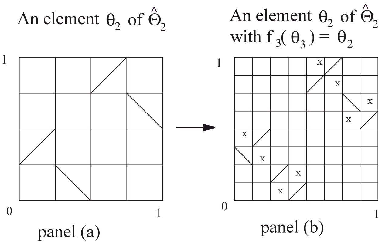
Let $N_{n}=\{0,1,2,...,2^{n}-1\}$. There are two equivalent representations of the automorphisms in $\hat{\Theta}_{n}.$ First representation involves a pair of functions, $\pi _{n}$ and $\mathcal{O}_{n}$ where $\pi _{n}:N_{n}\to N_{n}$ is a permutation of $N_{n}$ and $\mathcal{O}_{n}:N_{n}\to \{-1,1\}$ is a map as follows: For each $k\in N_{n},$ $\pi _{n}(k)$ specifies which subinterval of the unit interval the image of the $k^{th}$ subinterval be mapped to, and $\mathcal{O}_{n}\circ \pi _{n}(k)$ specifies the slope of the automorphism that the image subinterval will take. Denote such an automorphism as described above by the symbol

$$\theta _{n}=\left( \pi _{n}(k),\mathcal{O}_{n}\circ \pi _{n}(k)\right) _{k=0}^{2^{n}-1}. \tag{6}$$ The second representation of the above automorphism is the following:

$$\theta _{n}(x)=\left\{ \begin{array}{cc} \frac{\pi _{n}^{{}}(k)}{2^{n}}-\frac{k}{2^{n}}+x & \text{ if } x\in I_{k} \text{ and } \mathcal{O}_{n}(\pi _{n}(k))=+1 \\ & \\ \frac{\pi _{n}(k)+1}{2^{n}}-\frac{k}{2^{n}}-x & \text{ if } \in I_{k} \text{ and } \mathcal{O}_{n}(\pi _{n}(k))=-1 \\ & k=0,1,...2^{n}-1. \end{array} \right. \tag{7}$$ The notation $\theta _{n}$ will be used to mean the representation Equation 6 and the notations $\theta _{n}(.)$ or $\theta _{n}(x)$ will be used to mean the representation Equation 7 of an element in $\hat{\Theta}_{n}$. To illustrate further, an automorphism $\theta _{2}(x)$ corresponding to the permutation $\pi _{2}(1)=2$, $\pi _{2}(2)=1$, $\pi _{2}(3)=4$ and $\pi _{2}(4)=3$, and the slope map $\mathcal{O}_{2}(1)=-1$, $\mathcal{O}_{2}(2)=+1$, $\mathcal{O}_{2}(3)=-1$, and $\mathcal{O}_{2}(4)=+1$ is drawn in panel (a) of Figure 1.

For all $n\ge 0$, the finite subgroups $\hat{\Theta}_n$ of $\mathcal{G}$ are defined recursively as follows:

For $n=0$, there is no subdivision of $I,$ and take $$\hat{\Theta}_{0}=\left\{ \theta _{0}=(\pi _{0}(0),\mathcal{O}_{0}(0)) \mathcal{O}_{0}(0)\in \left\{ -1,1\right\} \right\} .$$ Note that $\hat{\Theta}_{0}$ has only two elements. To define $\hat{\Theta}_{1}$, notice that there are two dyadic sub-intervals of $I$ denoted as $I_{0}$ and $I_{1}$. Each $\theta _{0}\in \hat{\Theta}_{0}$, induces a unique permutation $\pi _{1,\theta _{0}}$ of $N_{1}=\{0,1\}$ defined by $$\pi _{1,\theta _{0}}(j)=i \text{ if for all }x\in I_{j}, \theta _{0}(x)\in I_{i}, i,j\in N_{1}.$$ For each $\theta _{0}\in \hat{\Theta}_{0}$ denote by $$A_{1}(\theta _{0})=\left\{ \theta _{1}=\left( \pi _{1,\theta _{0}}(k),\mathcal{O}_{1}(\pi _{1,\theta _{0}})(k)\right) _{k=0}^{1} \mathcal{O}_{1}(\pi _{1,\theta _{0}})(j)\in \left\{ -1,1\right\} ,j=0,1\right\} .$$ Define $\hat{\Theta}_{1}$to be the set $$\hat{\Theta}_{1}=\bigcup_{\theta _{0}\in \hat{\Theta}_{0}}A_{1}(\theta _{0}).$$ Note that each $A_{1}(\theta _{0})$ has $2\times 2=4$ elements and hence $\hat{\Theta}_{1}$ has $2\times 4=8$ elements. Suppose now that $\hat{\Theta}_{n-1}$ is already defined. Construct $\hat{\Theta}_{n}$ from $\hat{\Theta}_{n-1}$ as follows: Denote the $2^{n}$ dyadic sub-intervals at stage $n$ be denoted as $I_{0},$… $I_{2^{n-1}}$. Each $\theta _{n-1}\in \hat{\Theta}_{n-1}$ induces a unique permutation $\pi _{n,\theta _{n-1}}$ of the set $N_{n}$ defined by

$$\pi _{n,\theta _{n-1}}(j)=i\text{ if for all }x\in I_{j}, \theta _{n-1}(x)\in I_{i}, i,j\in N_{n}. \tag{8}$$ For each $\theta _{n-1}\in \hat{\Theta}_{n-1}$ define

$$A_{n}(\theta _{n-1})=\left\{ \begin{array}{l} \theta _{n}=\left( \pi _{n,\theta _{n-1}}(k),\mathcal{O}_{n}(\pi _{n,\theta _{n-1}})(k)\right) _{k=0}^{2^{n}-1} \\ \\ \mathcal{O}_{n}(\pi _{n,\theta _{n-1}})(i)\in \left\{ -1,1\right\} \forall i\in N_{n} \end{array} \right\} .$$ and $$\hat{\Theta}_{n}=\bigcup_{\theta _{n-1}\in \hat{\Theta}_{n-1}}A_{n}(\theta _{n-1}).$$

For each $n\ge 1$, define the projection maps $f_{n} : \hat{\Theta}_{n}\to \hat{\Theta}_{n-1}$,by $f_{n}(\theta _{n})=\theta _{n-1}$, where $\theta _{n-1}$ is related to $\theta _{n}$ by the requirement that $\theta _{n}\in A_{n}(\theta _{n-1})$. To get an idea about these projection maps, in panel (b) of Figure 1 a $\theta _{3}\in \hat{\Theta}_{3}$ is shown and its projection using the map $f_{3}$ is $\theta _{2}\in \hat{\Theta}_{2}$ which is shown in panel (a) of the figure.

Denote by $$\breve{\Theta}=\left\{ \breve{\theta}=(\theta _{0},\theta _{1},\theta _{2},....) \theta _{n}\in \hat{\Theta}_{n},\forall n\ge 0\text{ and } f_{n}(\theta _{n})=\theta _{n-1},\forall n\ge 1\right\}.$$ For any two elements $\breve{\theta}=(\theta _{0},\theta _{1},\theta _{2},....)$ and $\breve{\theta}^{\prime }=(\theta _{0}^{\prime },\theta _{1}^{\prime },\theta _{2}^{\prime },....)$ from $\breve{\Theta}$, define the multiplication operation $\breve{\theta}\circ \breve{\theta}^{\prime }$ by

$$\breve{\theta}\circ \breve{\theta}^{\prime }=\left( \theta _{0}\theta _{0}^{\prime },\theta _{1}\theta _{1}^{\prime },\theta _{2}\theta _{2}^{\prime },...\right)$$

With $\breve{\theta}^{-1}=(\theta _{0}^{-1},\theta _{1}^{-1},\theta _{2}^{-1},....)$ as the inverse of $\breve{\theta}=(\theta _{0},\theta _{1},\theta _{2},....)$, and with $\breve{e}=(e_{0},e_{1},...)$, where $e_{n}$ is the identity element of $\hat{\Theta}_{n}$ as the unit element, note that $\breve{\Theta}$ is a group. Define for $n\ge 0$ the projection maps $\pi _{n}:\breve{\Theta}\to \hat{\Theta}_{n}$ by

$$\pi _{n}(\breve{\theta})=\theta _{n}, \text{where} \breve{\theta}=(\theta_{0},\theta_{1},\theta _{2},....)$$

Let $\mathcal{F}=\cup _{n=1}^{\infty }\pi _{n}^{-1}\left( \mathcal{B}_{n}\right)$. It can be easily shown that $\mathcal{F}$ is a Boolean algebra. Let $\breve{\mathcal{B}}$ be the $\sigma -$algebra generated by $\mathcal{F}$. The measure space $\left( \breve{\Theta},\breve{\mathcal{B}}\right)$ is called the projective limit of the sequence of measure spaces, $(\hat{\Theta}_{n}\mathcal{B}_{n})$, $n\ge 0$ through the maps $f_{n},n\ge 1$. The following theorem is proved in Raut (1997).

Theorem 2 [Raut (1997)]

There exists a unique right invariant probability measure, $\breve{\Gamma}$ on the projective limit $(\breve{\Theta},\breve{\mathcal{B}})$ of the sequence of measurable groups $\left( \hat{\Theta}_{n},\mathcal{B}_{n},\Gamma _{n}\right) _{0}^{\infty }$ through the sequence of homomorphisms $\left\{ f_{n}\right\} _{0}^{\infty }$ such that

• (i ) $\breve{\Gamma}\pi _{n}^{-1}=\Gamma _{n}.$

• (ii ) $\left( \breve{\Theta},\breve{\mathcal{B}},\breve{\Gamma}\right)$ is an uncountably large separated probability measurable group.

• 3. For each $\breve{\theta}=(\theta _{0},\theta _{1},...,\theta _{n},...)\in \breve{\Theta}$, the limit $\breve{\theta}(t)=\lim_{n\to \infty }\theta _{n}(t)$ exists for all $t\in I$ and the limit function $\theta :I\to I$ is a Lebesgue measure preserving automorphism.

Two measure spaces, $\left( X_{i},\mathcal{B}_{i},\mu _{i}\right)$, $i=1,2$ are said to be isomorphic if there exists two sets $N_{i}\subset X_{i}$, $\mu _{i}(N_{i})=0$, $i=1,2$ and a Borel automorphism $T:X_{1}\backslash N_{1}\to X_{2}\backslash N_{2}$ such that $\mu _{1}T^{-1}=\mu _{2}$. In this paper I prove the following isomorphism theorem for the invariant probability measurable group $\left( \breve{\Theta},\breve{\mathcal{B}},\breve{\Gamma}\right)$.

Theorem 3 [Isomorphism Theorem] The projective limit group $\left(\breve{\Theta},\breve{\mathcal{B}},\breve{\Gamma}\right)$ is isomorphic to the unit interval with Lebesgue measure, $\left(I,\mathcal{B}_{I},\lambda \right)$.

Proof. Let $L_{2}(I)$ be the Hilbert space of square integrable functions with respect to the Lebesgue measure on $(I,\mathcal{B}_{I})$. Let $\mathcal{U}$ denote the set of all operators $U$ on $L_{2}(I)$ such that $U$ is onto and $U$ is isometric, i.e. $(U(f),U(g))=(f,g)$, $f,g\in L_{2}(I)$ where $(,)$ is the inner-product operation of $L_{2}(I)$. Such an operator $U$ of $L_{2}(I)$ is known as unitary operator. It is known that with respect to the strong operator topology, i.e., metric of the Banach space of bounded operators on $L_{2}(I)$, $\mathcal{U}$ is a complete, separable metric space. Each Lebesgue measure preserving automorphism $\theta$ defines a unitary operator $U(\theta )\in \mathcal{U}$ by $\left( U(\theta )f\right) (x)=f\left( \theta (x)\right) , f\in L_{2}(I)$. A Borel space is said to be standard if it is Borel isomorphic to the Borel space of a Borel measurable subset of a complete separable metric space. Thus, each $\left( \hat{\Theta}_{n},\mathcal{B}_{n},\Gamma _{n}\right)$ is standard and hence their countable Cartesian product $\left( \breve{\Theta},\breve{\mathcal{B}}, \breve{\Gamma}\right)$ is also standard (see Mackey (1957), Theorem 3.1). Notice that for any $\breve{\theta}=\left( \theta _{0},\theta _{1},...,\theta _{n},...\right) \in \breve{\Theta}$, we have $\left\{ \breve{\theta}\right\} =\lim_{n\to \infty }\pi _{n}^{-1}(\theta _{n})$. Hence $\breve{\Gamma}\left( \{\breve{\theta}\}\right) =\lim_{n\to \infty }\breve{\Gamma}\pi _{n}^{-1}(\theta _{n})=\lim_{n\to \infty }\Gamma _{n}\left( \{\theta _{n}\}\right) =0$, for all $\breve{\theta}\in \breve{\Theta}$. Thus, $\left( \breve{\Theta},\breve{\mathcal{B}},\breve{\Gamma}\right)$ is isomorphic to $\left( I,\mathcal{B}_{I},\lambda \right)$ (see Parthasarathy (1977).

$\blacksquare$

I utilize the above two theorems to derive a diagonal formula for the random order value operator with respect to the projective limit group $\breve{\Theta}$ on a larger class of games than it was shown in Raut (1997), and also use these results to prove Theorem 4 and Theorem 5 below.

4.2 The existence and uniqueness of $\breve\Theta$-symmetric random order value operator on $NBV$

Theorem 4 There exists a unique $\breve{\Theta}$-symmetric random order value operator $\Phi_{\breve{\Gamma}}$ on NBV.

Proof. Let $V\in \text{NBV}$. Let $S\in \mathcal{B}_{I}$ be an arbitrarily fixed coalition. By Proposition 3(i), the measure $\left( \phi ^{\breve{\theta}}V\right) (S)$ exists for all $\breve{\theta}\in \breve{\Theta}$. Denote by $h(\breve{\theta})\equiv \left( \phi ^{\breve{\theta}}V\right) (S)$. I want to show that $h$ is integrable with respect to the invariant probability measurable group $\left( \breve{\Theta},\breve{\mathcal{B}},\breve{\Gamma}\right)$. To that end, for any $\breve{\theta}=\left( \theta _{0},\theta _{1},...,\theta _{n},\theta _{n+1},..\right) \in \breve{\Theta}$, define a sequence $\breve{\theta}_{n}$, $n\ge 0$ of elements in $\breve{\Theta}$ by $\breve{\theta}_{n}\equiv \left( \theta _{0},\theta _{1},...,\theta _{n},\theta _{n}...\right)$, and for any function $h:\breve{\Theta}\to {\Re }$, define a sequence of functions, $h_{n}:\breve{\Theta}\to {\Re }$ by $h_{n}(\breve{\theta})\equiv h(\breve{\theta}_{n})$. It is then clear that $\lim_{n\to \infty }h_{n}(\breve{\theta})=h(\breve{\theta})$ for all $\breve{\theta}\in \breve{\Theta}$. It is also clear that $h_{n}(\breve{\theta})$ is $\pi _{n}^{-1}\left( \mathcal{B}_{n}\right)$ measurable, and hence $h_{n}(\breve{\theta})$ is measurable with respect to $\left( \breve{\Theta},\breve{\mathcal{B}}\right)$ for all $n\ge 0$. Furthermore, $$h_{n}(\breve{\theta}) = (\phi ^{\breve{\theta}_{n}}V)(S) \le \Vert \phi ^{\breve{\theta}_{n}}V\Vert _{BV}\le \Vert V\Vert _{BV}.$$ Thus by the Lebesgue’s dominated convergence theorem, the function $h(\breve{\theta}),$ which is the point-wise limit of a sequence of measurable functions dominated by a constant, is integrable with respect to $\left(\breve{\Theta},\breve{\mathcal{B}},\breve{\Gamma}\right)$.

The uniqueness of $\Phi _{\breve{\Gamma}}$ follows from Theorem 1.

$\blacksquare$

What kind of randomization pattern does the projective limit group render? To examine it, let pNA$\left( \mu \right)$ be the linear space of games generated by the polynomials of the non-atomic probability measure $\mu$ on the unit interval $I.$ Fix a $t\in I$ and an integer $n\ge 0$. Suppose $t\in I_{1}$. Consider the initial segments of player $t$ in each of the random orders $\theta _{n}\in \hat{\Theta}_{n}$, that has the same value for $t$, say $\theta _{n}(t)=t_{0}$. From Figure 1 it is clear that all these random orders place before player $t$ a particular type of sets of Lebesgue measure $t_{0}$. The type of the sets depends on $t_{0}$, and $n$. For example, suppose $t_{0}<1/2$, then all these random orders do not place any players from the interval $[1/2,1]$. Thus, the random orders in $\breve{\Theta}$ allow a player $t$ to form coalitions with sets of players of any size $t_{0},$ $0\le t_{0}\le 1$ but not all sets of players of a given size $t_{0}.$ Therefore, for games in which the worth of a coalition depends only through its size (in the Lebesgue measure sense) but not through any of their other identities, i.e., for anonymous games such as the games in pNA$\left( \lambda \right)$, one can expect that the expected marginal contribution of a player with respect to the group of random orders $\left( \breve{\Theta},\breve{\mathcal{B}},\breve{\Gamma}\right)$ coincides with the fully symmetric Aumann and Shapley axiomatic value.

For general non-atomic games of the form $f\circ \mu ,$ $\mu \in NA^{1},$ the $\breve{\Theta}$-symmetric random order value will not in general coincide with the fully symmetric value. But the procedure could be modified to produce the fully symmetric random order value as follows: For a general non-atomic measure $\mu$ it is known from the isomorphism theorem of measure theory (see for instance, Proposition 26.6 in Parthasarathy (1977)) that there exists a $\xi \in \mathcal{G}$ such that $\mu \xi ^{-1}=\lambda$. For games of this form, I take the set of orders to be the orders generated by the set of automorphisms $\breve{\Theta}_{\mu }\equiv \left\{ \theta \xi |\theta \in \breve{\Theta}\right\} .$ Note that $\breve{\Theta}_{\mu }$ is a translation of $\breve{\Theta}.$ I induce an invariant measure structure on the homogeneous space $\breve{\Theta}_{\mu }$ from the invariant measure structure of $\left( \breve{\Theta},\breve{\mathcal{B}},\breve{\Gamma}\right)$ using the one-one and onto map $\breve{\theta}\longmapsto \breve{\theta}\xi$ between $\breve{\Theta}$ and $\breve{\Theta}_{\mu }$. Denote the corresponding measure space as $\left( \breve{\Theta}_{\mu },\breve{\mathcal{B}_{\mu }},\breve{\Gamma}_{\mu }\right)$. We then have the following result.

Theorem 5 Let $f:I\to {\Re }$ be an absolutely continuous function, and let $\mu$ be a non-atomic probability measure on $I$. The unique $\breve{\Theta}_{\mu }$-symmetric random order value of the scalar measure game $f\circ \mu$ yields the following diagonal formula: $$\Phi _{\breve{\Gamma}_{\mu }}[f\circ \mu ](S)=\mu (S)\int_{0}^{1}f^{\prime }(t)d\lambda (t). \tag{9}$$ Thus, the $\breve\Theta_\mu$-symmetric random order value operator $\Phi _{\breve\Gamma}$ coincides with the Aumann-Shapley axiomatic value operator on all of $pNA\left( \mu \right)$.

Proof. Note that in the case of $\mu =\lambda ,$ $$\begin{aligned} \Phi _{\breve{\Gamma}}(f\circ \lambda )(S) &=\int_{\breve{\Theta}}\left( \phi ^{\breve{\theta}}(f\circ \lambda )\right) (S)d\breve{\Gamma}(\breve{\theta}) \\ &=\int_{\breve{\Theta}}\int_{S}f^{\prime }(\breve{\theta}(t))d\lambda (t)d \breve{\Gamma}(\breve{\theta}),\text{ ...(1) } \\ &=\int_{S}\left[ \int_{\breve{\Theta}}f^{\prime }(\breve{\theta}(t))d\breve{\Gamma}(\breve{\theta})\right] d\lambda (t),\text{ by the Fubini's Theorem} \\ &=\int_{S}\left[ \int_{0}^{1}f^{\prime }(x)d\lambda (x)\right] d\lambda (t),\text{ ... (2)} \\ &=\lambda (S)\int_{0}^{1}f^{\prime }(x)d\lambda (x). \end{aligned}$$ In the above, the step (1) follows from Equation 5 and step (2) follows from Theorem 3 and the fact that $f^{\prime }\in L_{1}(I)$. Note that for any $\xi \in \mathcal{G}$, $\Phi _{\breve{\Gamma}}\left( \xi ^{*}\left( f\circ \lambda \right) \right) (S)$ $=\Phi _{\breve{\Gamma} }\left( f\circ \lambda \right) \left( \xi ^{-1}(S)\right)$ $=\lambda \left( \xi ^{-1}(S)\right) \int_{0}^{1}f^{\prime }(x)dx$ $=\xi ^{*}\Phi _{\breve{ \Gamma}}\left( f\circ \lambda \right) (S)$. Thus $\breve{\Theta}$-symmetric random order value of a game of the form $(f\circ \lambda )(S)$ is symmetric with respect to the full group of automorphisms, $\mathcal{G}$.

For the general non-atomic measure $\mu ,$ note that for any order $\bar{ \theta}=\theta \xi \in \breve{\Theta}_{\mu },$ we have $$\begin{aligned} \phi ^{\bar{\theta}}\left( f\circ \mu \right) \left( S\right) &=\phi ^{\theta \xi }\left( f\circ \mu \right) \left( \xi ^{-1}\xi \left( S\right) \right) \\ &=\phi ^{\theta }\left( \ddot{\xi}\left( f\circ \mu \right) \right) \left( \xi \left( S\right) \right) \text{ ... (1) } \\ &=\phi ^{\theta }\left( f\circ \lambda \right) \left( \xi \left( S\right) \right) \\ &=\int_{\xi \left( S\right) }f^{\prime }\left( \theta \left( t\right) \right) d\lambda \left( t\right) \text{... (2).} \end{aligned}$$ In the above, the step (1) follows from Equation 4 and the step (2) follows from Equation 5. Hence, $$\begin{aligned} \Phi _{\breve{\Gamma}_{\mu }}(f\circ \mu )(S) &=\int_{\breve{\Theta}_{\mu }}\phi ^{\bar{\theta}}\left( f\circ \mu \right) \left( S\right) d\breve{ \Gamma}_{\mu }(\bar{\theta}) \\ &=\int_{\breve{\Theta}_{\mu }}\left[ \int_{\xi (S)}f^{\prime }(\theta \left( t\right) )d\lambda \left( t\right) \right] d\breve{\Gamma}_{\mu }( \bar{\theta}) \\ &=\int_{\xi \left( S\right) }\int_{\breve{\Theta}}f^{\prime }\left( \theta \left( t\right) \right) d\breve{\Gamma}(\theta \grave{)}d\lambda \left( t\right) ,\text{ by the Fubini's Theorem} \\ &=\int_{\xi \left( S\right) }d\lambda \left( t\right) \int_{0}^{1}f^{\prime }(x)dx \\ &=\mu (S)\int_{0}^{1}f^{\prime }(x)dx. \end{aligned}$$

$\blacksquare$

5 Further Remarks

Remark R1: There are economically important non-smooth games which neither belong to bv$^{\prime }$NA, MIX, nor even to ASYMP. Mertens (1988) extended the diagonal formula for the value to a very powerful closed subspace of games in BV, known as Mertens space, on which the extended diagonal formula provides a value operator of norm 1 and the Mertens space was shown to include all well known spaces such as bv$^{\prime}$NA, ASYMP, DIFF and DIAG. J.F. Mertens and Abraham Neyman suggested to me to explore if the Mertens space belongs to $L1(\breve{\Theta},\breve{\Gamma})$. I have not tried to get a general answer to this question, instead I show that the $\breve{\Theta}$-symmetric random order value exists for the non-smooth game of n-handed gloves marketsconsidered in example 19.2 of Robert J. Aumann and Shapley (1974) : $V(S)=\min \left\{ \mu _{1}(S),\mu _{2}(S),...,\mu _{n}(S)\right\}$, $\mu _{i}\in NA$$^{1}$, $i=1,2,...n,$ and $S\in B_{I}$. This kind of non-smooth games arise in economies with strong complementarities. Aumann and Shapley showed that this game did not belong even to ASYMP when $n>2$. One of the motivations for Mertens (1988) to extend the diagonal formula to the Mertens space was to include such games in the space. Notice that V is of bounded variation. Since each $\mu _{i}$ is a non-atomic probability measure, the game $V(S)$ is normalized and hence belongs to NBV. Thus there exists a unique $\breve{\Theta}$-symmetric random order value for V.

Remark R2: An important issue regarding the reformulated random order approach of this paper is: What characteristics of the group $\breve{\Theta}$ that makes the random order value coincides with the axiomatic value on pNA($\lambda$)? In Section 2, I argued that a random order generated according to the probability model $\left( \breve{\Theta},\breve{\mathcal{B}},\breve{\Gamma}\right)$ has the characteristics that the random set of players that is placed before any given player is equally likely to be of any size $s\in \lbrack 0,1]$; for anonymous games in which the worth of a coalition depends only through its size not names such as games in pNA($\lambda)$, each player gets the average of the set of all possible marginal contributions with coalitions of all possible sizes, and thus the average is fully symmetrized in the sense that the value thus obtained is symmetric with respect to the full group of automorphisms. Locally finite groups of automorphisms may not do the job, as I have illustrated in Section 2. The games that arise in most economic applications are anonymous. However, for a wider applicability of the present approach, we must construct a larger invariant probability measurable group structure than $\left( \breve{\Theta},\breve{\mathcal{B}},\breve{\Gamma}\right)$, so that the random order value $\Phi _{\breve{\Gamma}}(V)$ with respect to it also fully symmetrizes many non-anonymous games.

Remark R3: Robert Aumann pointed out to me that for an alternative reformulation of random order approach to value, one might give up the measure theoretic model of the player set, i.e., $\left( I,\mathcal{B}_{I}\right)$, and consider instead a torus or other topological spaces with more well-behaved automorphism groups as the player space. It should be noted that there can exist only two orders on any topological space that is connected. This, for instance, will greatly simplify our analysis of random order value. I do not know, however, what kind of fairness such a symmetry group entails and what kind of economic situations are appropriate for such models; most of the economic models with a continuum of agents, however, have employed a measure theoretic structures on the space of agents, and thus we must begin to imagine the nature and study the implications of economic models with a topological space of agents.

Remark R4: If the set $\Theta$ is taken to be the full automorphism group $G$, then the existence of an Aumann-Shapley axiomatic value operator on $pNA$ can be reduced to the question of the existence of an invariant probability measurable group structure, $\left( \mathcal{G},\mathcal{B},\Gamma \right)$, with the property that $pNA\subset L1(G,\Gamma)$. Could one circumvent the Impossibility Principle of Aumann and Shapley in this reformulated approach? Indeed, on any group $\Theta$, there always exists a right invariant probability measurable group structure, for instance, the trivial, coarsest $\sigma$-algebra, $B=\left\{ \emptyset ,\Theta \right\}$ with a trivial probability measure that assigns $0$ to empty set and 1 to the whole set. The coarser the $\sigma$-algebra is, the meager are the sets of measurable and integrable functions, and hence fewer games belong to $L1(\Theta ,\Gamma )$ which may not include games in pNA. I guess the proof of Aumann-Shapley impossibility theorem could be adopted to the present framework to produce a negative answer to the above question. Very little is known about the structure of the group $G$ that can shed light on the above issues, and I have not pursued these issues any further in this paper.

I keep the above unresolved issues for future research to shed more light on.

References

Aumann, Robert J. 1967. “Random Measure Preserving Transformations.” Shapley Value. In Proceedings of the Fifth Berkeley Symposium on Mathematical Statistics and Probability, 2:321–26. Part II. L. M. LeCam; J. Neyman, University of California Press. http://digitalassets.lib.berkeley.edu/math/ucb/text/math_s5_v2_p2_article-21.pdf.

Aumann, Robert J., and Lloyd S. Shapley. 1974. Values of Non-Atomic Games. Shapley Value. Princeton University Press.

Halmos, Paul Richard. 1950. Measure Theory. Vol. 2. van Nostrand New York. https://doi.org/10.1007/978-1-4684-9440-2.

Kannai, Yakar. 1966. “Values of Games with a Continuum of Players.” Israel Journal of Mathematics 4 (1): 54–58. https://doi.org/10.1007/bf02760070.

Mackey, George W. 1957. “Borel Structure in Groups and Their Duals.” Trans. Amer. Math. Soc. 85 (1): 134–65. https://doi.org/10.1090/s0002-9947-1957-0089999-2.

Mertens, J. F. 1988. “The Shapley Value in the Non Differentiate Case.” Int J Game Theory 17 (1): 1–65. https://doi.org/10.1007/bf01240834.

Monderer, D. 1989. “Weighted Majority Games Have Many $\mu$-Values.” Int J Game Theory 18 (3): 321–25. https://doi.org/10.1007/bf01254295.

Monderer, Dov. 1986. “Measure-Based Values of Nonatomic Games.” Mathematics of Operations Research 11 (2): 321–35. https://doi.org/10.1287/moor.11.2.321.

Monderer, Dov, and William H. Ruckle. 1990. “On the Symmetry Axiom for Values of Nonatomic Games.” International Journal of Mathematics and Mathematical Sciences 13 (1): 165–69. https://doi.org/10.1155/s0161171290000229.

Neyman, Abraham. 2002. “Chapter 56 Values of Games with Infinitely Many Players.” Handbook of Game Theory with Economic Applications Volume 3, 2121–67. https://doi.org/10.1016/s1574-0005(02)03019-9.

Parthasarathy, Kalyanapuram Rangachari. 1977. “Introduction to Probability and Measure.”

Raut, Lakshmi K. 1997. “Construction of a Haar Measure on the Projective Limit Group and Random Order Values of Non-Atomic Games.” Published. Journal of Mathematical Economics 27 (2): 229–50. https://doi.org/10.1016/s0304-4068(96)00753-7.

———. 2003. “Symmetry Axiom and Haar Measure for Random Order Shapley Value of Games.” Working: Shapley Value. Working Paper.

Ruckle, William H. 1982. “Projection in Certain Spaces of Set Functions.” Mathematics of Operations Research 7 (2): 314–18. https://doi.org/10.1287/moor.7.2.314.

Rudin, W. 1987. Real and Complex Analysis. McGraw-Hill, New York.

Segal, I. E., and R. A. Kunze. 1968. Integrals and Operators. New Delhi: Tata McGraw-Hill Publishing Company Ltd., New Delhi.

Shapley, Lloyd S. 1953. “A Value for n-Person Games.” Technical report. Contributions to the Theory of Games.

Footnotes

1. For other recent developments in axiomatic value, see Neyman (2002).

2. In the finite players case an automorphism is known as permutation.

3. When $\Theta$ is a locally compact topological group, and $\mathcal{A}$ is the Borel $\sigma$-algebra, such that $\Gamma (U)>0$, for every non-empty open set $U\subset \Theta$, then the Borel measure $\Gamma$ is known as the Haar Measure.

4. N is a normal subgroup of a group G if for all $\theta \in \text{G}$, we have $\theta ^{-1}\nu \theta \in \text{N}$ for all $\nu \in \text{N}$.

5. The Borel isomorphism theorem states that for any two sets of the same cardinality if both sets are Borel subsets of complete and separable metric spaces, then there exists a Borel isomorphism between these two sets, i.e., there exists a one-one and onto map between the sets such that both the map and its inverse are Borel measurable with respect to the relative Borel $\sigma$-algebras of the sets. Notice that both $I$ and $I\cup \{2\}$ are Borel subsets of $\Re$, hence there exists a Borel isomorphism between these two sets.

6. This is also referred as order complete and it is distinct from the completeness axiom used in defining preference relation in the utility theory.

7. I am grateful to Professor Robert Aumann for drawing my attention to this result.

8. This separation notion for measurable groups is the analogue of the Hausdorff separation axiom for topological spaces, see Halmos (1950), p.273.